Figures

Any figure that you create with code in your .Rmd document will be inserted inline into your knitted output file. Previously, we learned about how the knitr package is responsible for both executing code and knitting the output back into the document. When a code chunk produces a figure, knitr has some special code chunk options to control how your figure looks.

The author makes the graph, saves it as a file, and then copy and pastes it into the final report. This process relies on manual labor. If the data changes, the author must repeat the entire process to update the graph.

Naming figures

also covered:

Organize your code with knitr chunk labels (kebabs, not snakes)
setup chunk for setting global options (+ fig.path!)

Saving figures

Figure placement

By default, plots show up immediately after the code that prints them.

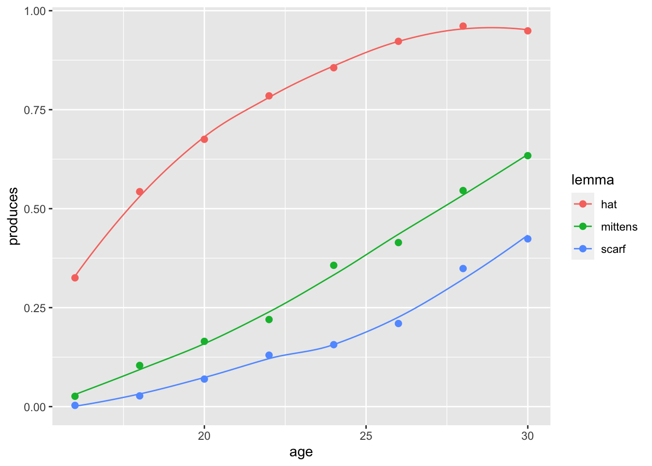
For example, the following line plot created with the ggplot2 package will be inserted when you knit.

ggplot(words, aes(x = age, y = produces, color = lemma)) + 
  geom_smooth(se = FALSE, lwd = .5) +
  geom_point(size = 2)

By contrast, the code chunk on the right will create a plot object named line.

If you ran this code in your console, it would not print the plot until you call the line object by name. The same will be true when you knit.

fig.align = 'center' / 'left' / 'right' aligns the figure in the output
fig.show = 'hide' / 'hold' hides plots entirely, or holds printing until end of a chunk

line <- 
  ggplot(words, aes(x = age, y = produces, color = lemma)) + 
  geom_smooth(se = FALSE, lwd = .5) +
  geom_point(size = 2)

line

Figure size

It can often be hard to get your figures to show up in the right size and place in your knitted output. Some knitr chunk options that help with this are:

out.width = '50%' allows you resize a plot (here, shrunk to half its original size; for full width, set to '100%')
fig.asp = 0.618 to control the ratio of height to width (this is the golden ratio, but any number will do: < 1 will be more wide than tall)

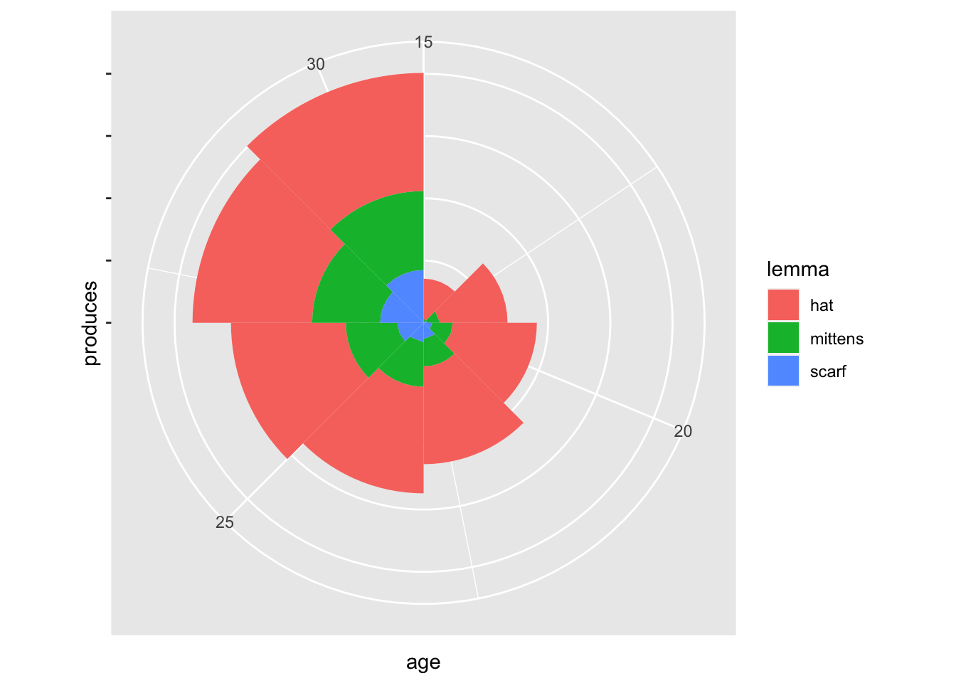
A neat trick you can use by combining these chunk options is to place two figures side-by-side:

```{r out.width='50%', fig.show='hold'}
plot1
plot2
```

line
rose

Figure captions & alt text

fig.cap = "Oh caption, my caption!" produces a figure caption; this will change the figure from inline to “floating”.
fig.alt = "Informative alt text" produces alt text for a figure, meant for screen readers.

hello

goodbye